On Linear Regressions
22 Jul 2018This blog post has a somewhat different target public: instead of focusing on the Machine Learning practician, it targets the Cognitive Science student who often uses Regression in his everyday statistics without understanding well how it works. Of course, there is a lot more to say than what is written here, but hopefully it will be a good basis upon which to build.
The Psycholinguistics group of the University of Kaiserslautern, where I am currently a PhD student, offered a course on Computational Linguistics this last Summer Semester1, where I had the opportunity to give three classes. I ended up writing a lot of material on Linear Regression (and some other stuff) that I believe would be beneficial not only for the students of the class, but for anyone else interested in the topic. So, well, this is the idea of this blog post…
In the class, we used Python to (try to) make things more “palpable” to the
students. I intend to do the exact same here. In fact, I am using
jupyter notebook for the first time along with this blog (if you are reading
this published, it is because it all went well). My goal with the Python codes
below is to make the ideas implementable also by the interested reader. If you
can’t read Python, you should still be able to understand what is going on by
just ignoring (most of) the code. Notice that most of the code blocks is
organized in two parts: (1) the part that has code, which is normally colorful,
highlighting the important Python words; and (2) the part that has the output,
which is normally just grey. Sometimes the code will also output an image
(which is actually the interesting thing to look at).
Still… for those interested in the Python, the following code loads the libraries I am using throughout this blog post:
# If you get a "No module named 'matplotlib'" error, you might have to
# install matplotlib before running this line. To do so, go to the
# terminal, activate your virtual environment, and then run
#
# pip install matplotlib

import matplotlib.pyplot as plt
from matplotlib import cm
from mpl_toolkits.mplot3d import axes3d
import pylab

# You might also need to install numpy. Same thing:
# pip install numpy
import numpy as np

# The same is true for sklearn:
# pip install sklearn
import sklearn
from sklearn import linear_model
Example Dataset
To make this easier to understand, we will create a very simple dataset. In this fictitious dataset, different participants read some sentences and had their eye tracked by a camera in front of them. Then, some parameters related to their readings were recorded.
Say our data looks like the following…
(notice that this data is COMPLETELY FICTITIOUS and probably DOES NOT reflect reality!)
# Generates some fictitious data

columns = ["gender",
           "mean_pupil_dilation",
           "total_reading_time",
           "num_fixations"]

data = [
    ['M',  0.90,  120,  20],
    ['F',  0.89,  101,  18],
    ['M',  0.79,  104,  24],
    ['F',  0.91,  111,  19],
    ['F',  0.77,   95,  20],
    ['F',  0.63,   98,  22],
    ['M',  0.55,   77,  30],
    ['M',  0.60,   80,  23],
    ['M',  0.55,   67,  56],
    ['F',  0.54,   63,  64],
    ['M',  0.45,   59,  42],
    ['M',  0.44,   57,  43],
    ['F',  0.40,   61,  51],
    ['F',  0.39,   66,  40]
]

test_data = [
    ['M',  0.87,  102,  17],
    ['F',  0.74,  101,  12],
    ['M',  0.42,   60,  52],
    ['F',  0.36,   54,  44]
]
For the non-Python readers, this dataset is basically composed of the following two tables.
- A Training Data (which will be normally referred to as
datain the codes below)
| Gender | Mean Pupil Dilation | Total Reading Time | Num Fixations |
|---|---|---|---|
| M | 0.90 | 120 | 20 |
| F | 0.89 | 101 | 18 |
| M | 0.79 | 104 | 24 |
| F | 0.91 | 111 | 19 |
| F | 0.77 | 95 | 20 |
| F | 0.63 | 98 | 22 |
| M | 0.55 | 77 | 30 |
| M | 0.60 | 80 | 23 |
| M | 0.55 | 67 | 56 |
| F | 0.54 | 63 | 64 |
| M | 0.45 | 59 | 42 |
| M | 0.44 | 57 | 43 |
| F | 0.40 | 61 | 51 |
| F | 0.39 | 66 | 40 |
- And a Test Data (
test_datain the codes below)
| Gender | Mean Pupil Dilation | Total Reading Time | Num Fixations |
|---|---|---|---|
| M | 0.87 | 102 | 17 |
| F | 0.74 | 101 | 12 |
| M | 0.42 | 60 | 52 |
| F | 0.36 | 54 | 44 |
Why do you have these two tables instead of one?
I won’t go into details here, but the way things work in Machine Learning is that you normally “train a model” using the Training Data and then you use this model to try to predict the values in the Test Data. This way you can make sure that your model is capable of predicting values from data that it has never seen.
In this blog post I won’t actually use the Test Data, but I thought it made sense to show it here so that the reader keeps in mind that this is the way he would actually check if the Regression model that is learnt below is capable of generalizing to new data, that has never been used before.
Defining Regression
If you look at our data, you will see that there seems to be a relation between the dilation of the pupil of a participant and his reading time. That is, a participant with high dilation seems to have longer reading times than a participant with low dilation. It might make sense, then, to pose the following question: is it possible to guess more or less the mean_pupil_dilation from the total_reading_time? Guessing the value of a continuous variable from the value of other continuous variables is what is known in Machine Learning as Regression.
In more formal terms, we will define Regression as follows. Given:
- An input space $I$.
- A dataset containing pairs $(d_i, l_i),~~i=1, \ldots, k$, where $d_i \in I$ and $l_i \in \mathbb{R}$.
Our goal was then to find a model $f: I \rightarrow \mathbb{R}$ that, given a new (unseen) $d$, is capable of predicting its correct $l$ (i.e., $f(d) = l$).
So… first thing… let’s plot mean_pupil_dilation and total_reading_time to see how they look like:
# Gets the data
# (the `astype()` call is because Python was taking the numbers as strings)
mean_pupil_dilation = np.array(data)[:, 1].astype(float)
total_reading_time  = np.array(data)[:, 2].astype(float)

# Let's show the data here too
print("mean_pupil_dilation", mean_pupil_dilation)
print("total_reading_time", total_reading_time)

# Creates the canvas
fig, axes = plt.subplots()

# Really plots the data
axes.plot(mean_pupil_dilation, total_reading_time, 'o')

# Puts names in the two axes (just for clearness)
axes.set_xlabel('Mean Pupil Dilation')
axes.set_ylabel('Total Reading Time')

pylab.xlim([0,1])
pylab.ylim([15, 125])
mean_pupil_dilation [0.9  0.89 0.79 0.91 0.77 0.63 0.55 0.6  0.55 0.54 0.45 0.44 0.4  0.39]
total_reading_time [120. 101. 104. 111.  95.  98.  77.  80.  67.  63.  59.  57.  61.  66.]
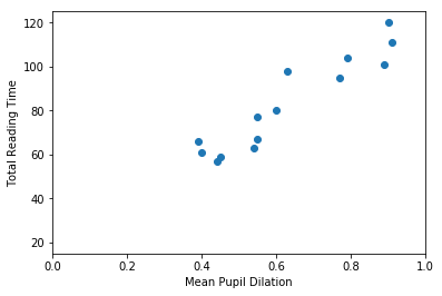
It should be quite visible that you can have a good guess (from this data) of one of the values based on the other. That is, that you can guess the Total Reading Time based on the Mean Pupil Dilation
Formulating the Problem
In this first example, our goal is to find a function that crosses all dots in the graph above. That is, this function should, for the values of mean_pupil_dilation that we know, have the values of total_reading_time in our dataset (or be the closest possible to them). We will also assume that this function is “linear”. That is, we assume that it is possible to find a single straight line that works as a soluton for our problem.
With these assumptions in hand, we can now define this problem in a more formal way. A line can be always described by the function $y = Ax + b$, where the $A$ is referred to as the slope, and $b$ is normally called the intercept (because it is where the line intercepts the $y$-axis when $x = 0$). In our case, the points that we already know about the line are going to help us to decide how this line is supposed to look like. That is:
\[\begin{cases} 66 &= A \cdot 0.39 &+ b \\ 61 &= A \cdot 0.4 &+ b \\ 57 &= A \cdot 0.44 &+ b \\ 59 &= A \cdot 0.45 &+ b \\ 63 &= A \cdot 0.54 &+ b \\ 67 &= A \cdot 0.55 &+ b \\ 80 &= A \cdot 0.6 &+ b \\ 77 &= A \cdot 0.55 &+ b \\ 98 &= A \cdot 0.63 &+ b \\ 95 &= A \cdot 0.77 &+ b \\ 111 &= A \cdot 0.91 &+ b \\ 104 &= A \cdot 0.79 &+ b \\ 101 &= A \cdot 0.89 &+ b \\ 120 &= A \cdot 0.9 &+ b \\ \end{cases}\]The equations above came directly from our table above. For one of the participants, when total_reading_time is 66, the mean_pupil_dilation is 0.39. For the next, when the total_reading_time is 61, the mean_pupil_dilation is 0.4. We make the total_reading_time the $y$ of our equation (the value that we want to predict), and it is predicted by a transformation of the mean_pupil_dilation (our $x$).
Of course, you don’t need to be a genius to realize that this system of equations has no solution (that is, that no straight line will actually cross all the points in our graph). So, our goal is to find the best line that gets the closest possible to all points we know. To indicate this in our equations, we insert a variable that stands for the “error”.
\[\begin{cases} 66 &= A \cdot 0.39 &+ b + \epsilon_1 \\ 61 &= A \cdot 0.4 &+ b + \epsilon_2 \\ 57 &= A \cdot 0.44 &+ b + \epsilon_3 \\ 59 &= A \cdot 0.45 &+ b + \epsilon_4 \\ 63 &= A \cdot 0.54 &+ b + \epsilon_5 \\ 67 &= A \cdot 0.55 &+ b + \epsilon_6 \\ 80 &= A \cdot 0.6 &+ b + \epsilon_7 \\ 77 &= A \cdot 0.55 &+ b + \epsilon_8 \\ 98 &= A \cdot 0.63 &+ b + \epsilon_9 \\ 95 &= A \cdot 0.77 &+ b + \epsilon_{10} \\ 111 &= A \cdot 0.91 &+ b + \epsilon_{11} \\ 104 &= A \cdot 0.79 &+ b + \epsilon_{12} \\ 101 &= A \cdot 0.89 &+ b + \epsilon_{13} \\ 120 &= A \cdot 0.9 &+ b + \epsilon_{14} \\ \end{cases}\]Now… this notation is quite cluttered with lots of variables that repeat a lot. People who actually do this normally prefer to write this with matrices. The following equation means exactly the same:
\[\begin{bmatrix} 66 \\ 61 \\ 57 \\ 59 \\ 63 \\ 67 \\ 80 \\ 77 \\ 98 \\ 95 \\ 111 \\ 104 \\ 101 \\ 120 \end{bmatrix} = A \begin{bmatrix} 0.39 \\ 0.4 \\ 0.44 \\ 0.45 \\ 0.54 \\ 0.55 \\ 0.6 \\ 0.55 \\ 0.63 \\ 0.77 \\ 0.91 \\ 0.79 \\ 0.89 \\ 0.9 \end{bmatrix} + b + \begin{bmatrix} \epsilon_{1} \\ \epsilon_{2} \\ \epsilon_{3} \\ \epsilon_{4} \\ \epsilon_{5} \\ \epsilon_{6} \\ \epsilon_{7} \\ \epsilon_{8} \\ \epsilon_{9} \\ \epsilon_{10} \\ \epsilon_{11} \\ \epsilon_{12} \\ \epsilon_{13} \\ \epsilon_{14} \\ \end{bmatrix}\]Finally… we often replace the vectors by bold letters and just write it as:
\[\mathbf{y} = A\mathbf{x} + b + \boldsymbol{\epsilon}\]Our goal is, then, for each of the equations above, to find values of $A$ and $b$ such that the $\epsilon_i$ (i.e., the error) associated with that equation is the minimum possible.
Evaluating a Regression solution
Now… there is a literally infinite number of possible lines, and we need to find a way to evaluate them, that is, decide if we like a certain line more than the others. For this, we probably should use the errors (i.e., the $\boldsymbol{\epsilon}$): lines that have big errors should be discarded, and lines that have low errors should be preferred. Unfortunately, there are several ways to “put together” all the $\epsilon_i$ denoting the errors associated with a given line. One way to “put together” all these $\epsilon_i$ could be summing them all:
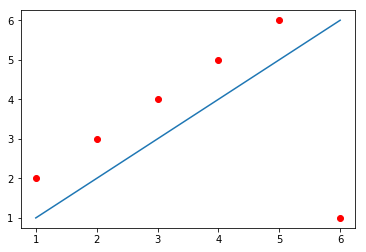
\[\text{Error over all equations: } \\E_{naïve} = \sum_i{\epsilon_i}\]However, you might have guessed by the word “naïve” there that this formula has problems. The problem with this formula the following: that, when some points are above and some points are below the line, the errors will “cancel” each other. For example, in the image below, the line does not cross any of the data points, but still produces an $E_{naïve} = 0$. How? The line passes at a distance of exactly 1 from the first five data points, producing a positive error (because the points are above the line) of 1 for each of them; but also passes at a distance of exactly 5 from the sixth data point, producing a negative error (because the point is below the line) of -5. When you sum up everything, you get $E_{naïve} = 1 + 1 + 1 + 1 + 1 - 5 = 0$.
X = [1,2,3,4,5,6]
Y_line = np.array([1,2,3,4,5,6])
Y_dots = np.array([2,3,4,5,6,1])

plt.plot(X, Y_line)
plt.plot(X, Y_dots, 'ro')
[<matplotlib.lines.Line2D at 0x7f1515f17b70>]
One solution to this problem could be to simply use the absolute value of each $\epsilon$ when calculating the error value:
\[\text{Error over all equations: } \\E_{L_1} = \sum_i{\mid\epsilon_i\mid} = \|\boldsymbol{\epsilon}\|_1\]This is a commonly used formula for evaluating the quality of a regression curve. Summing the magnitude of each $\epsilon$ this way is referred to as calculating the $L_1$ norm of the $\epsilon$ vector.
Unfortunately, the absolute-value function is not differentiable everywhere in its domain (that is, the derivative of this function is not defined at the point when $x = 0$ – if you don’t know what derivative or differentiation is, don’t worry, this is not super crucial for understanding the rest). This is not a terrible problem, but we are going to need differentiation later, and a great alternative function that doesn’t have this problem is the $L_2$ norm:
\[\text{Error over all equations: } \\E_{L_2} = \sum_i{ {\epsilon_i}^2} = \|\boldsymbol{\epsilon}\|_2 \\ \text{(}\textit{i.e.}\text{, the Sum of Squared Errors)}\]The code below shows each of the alternative errors for the simple example above, where, as we saw, the $E_{naïve} = 0$.
# (Following the example immediately above)

# Calculating the error in a very naive way
print("Error naive: ", np.sum(Y_dots - Y_line))

# Calculating the error using the absolute value of the epsilons:
print("Error L1:    ", np.sum(np.absolute(Y_dots - Y_line)))

# Calculating the error using the absolute value of the epsilons:
print("Error L2:    ", np.sum((Y_dots - Y_line)**2))
Error naive:  0
Error L1:     10
Error L2:     30
This last function (the $E_{L_2}$) is the usual choice for evaluating the Regression line. It is differentiable everywhere, but is not so robust to outliers as the $L_1$ norm.
Motivating Gradient Descent (a method to find the best line)
In the sections above, we have defined what we want to get: a good line – hopefully, the best one – that (almost) crosses all the points in our dataset. We have also understood how to decide if a line is good or not, based on the errors between the value predicted by the line and the value that appears in our data.
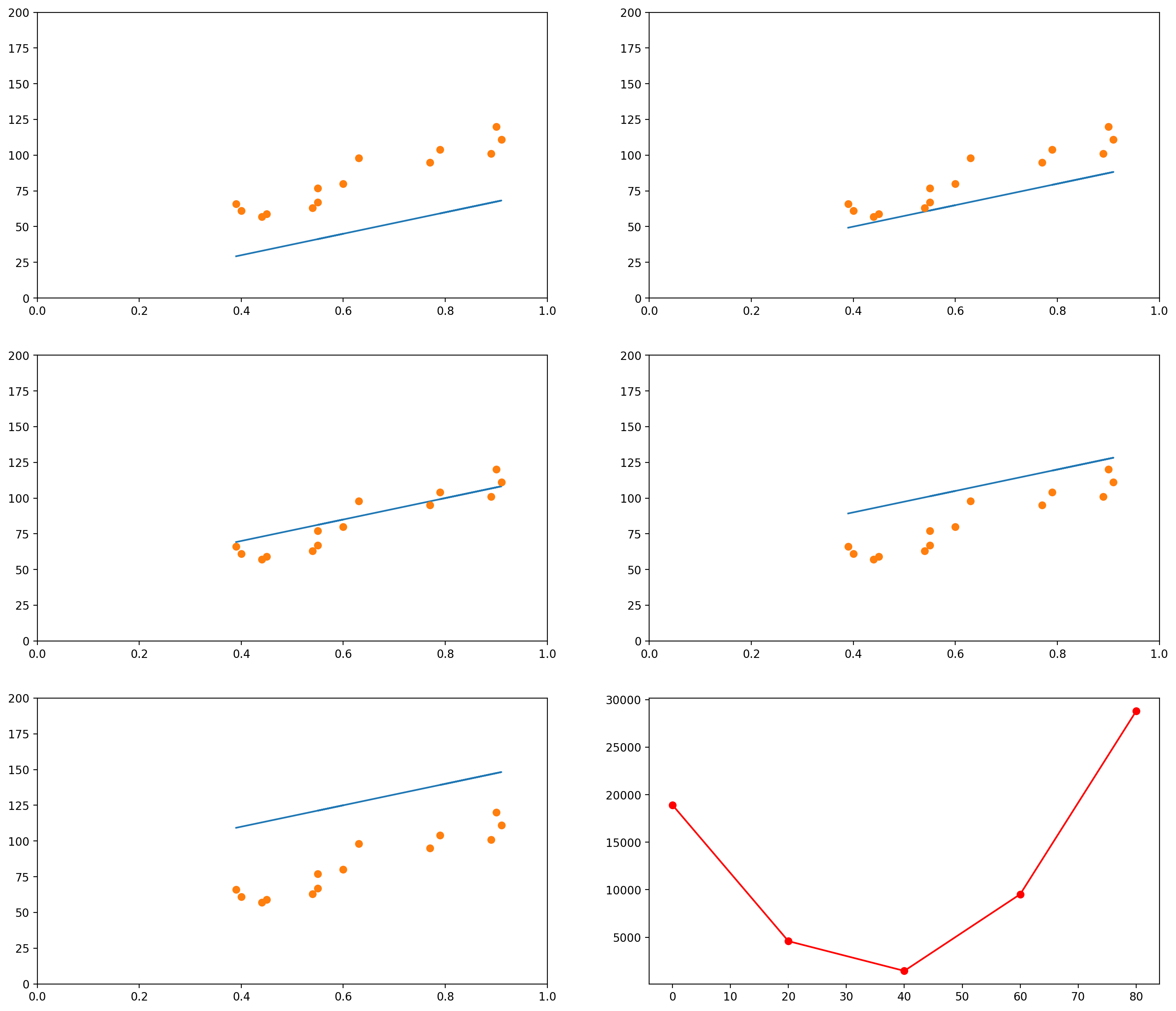
The images below show several possible lines, with an intercept of 0 and slopes 10, 30, 50, 100 and 200. The last graph shows the Sum of Squared Errors (the $L_2$ norm of the error vector $\epsilon$) for each of the lines:
# This is the original data
data_x = mean_pupil_dilation
data_y = total_reading_time

# Let's create some possible lines
plot_x1 = mean_pupil_dilation
plot_y1 = 10*plot_x1 + 0

plot_x2 = mean_pupil_dilation
plot_y2 = 30*plot_x2 + 0

plot_x3 = mean_pupil_dilation
plot_y3 = 50*plot_x3 + 0

plot_x4 = mean_pupil_dilation
plot_y4 = 100*plot_x4 + 0

plot_x5 = mean_pupil_dilation
plot_y5 = 200*plot_x5 + 0

# Now let's plot these lines, along with the data
def plot_line_and_dots(line, dots, lims):
    line_x, line_y = line
    dots_x, dots_y = dots
    xlim, ylim = lims
    plt.plot(line_x, line_y)
    plt.plot(dots_x, dots_y, 'o')
    plt.xlim(xlim)
    plt.ylim(ylim)

plt.figure(figsize=(18, 16), dpi= 200)

plt.subplot(3,2,1)
plot_line_and_dots([plot_x1, plot_y1], [data_x, data_y], [[0,1],[0, 200]])

plt.subplot(3,2,2)
plot_line_and_dots([plot_x2, plot_y2], [data_x, data_y], [[0,1],[0, 200]])

plt.subplot(3,2,3)
plot_line_and_dots([plot_x3, plot_y3], [data_x, data_y], [[0,1],[0, 200]])

plt.subplot(3,2,4)
plot_line_and_dots([plot_x4, plot_y4], [data_x, data_y], [[0,1],[0, 200]])

plt.subplot(3,2,5)
plot_line_and_dots([plot_x5, plot_y5], [data_x, data_y], [[0,1],[0, 200]])

# Finally, in the last plot, let's look at the error between the

squared_errors1 = (plot_y1 - total_reading_time)**2
squared_errors2 = (plot_y2 - total_reading_time)**2
squared_errors3 = (plot_y3 - total_reading_time)**2
squared_errors4 = (plot_y4 - total_reading_time)**2
squared_errors5 = (plot_y5 - total_reading_time)**2

plt.subplot(3,2,6)
plt.plot([10, 30, 50, 100, 200],
         [sum(squared_errors1),
          sum(squared_errors2),
          sum(squared_errors3),
          sum(squared_errors4),
          sum(squared_errors5)], '-ro')
[<matplotlib.lines.Line2D at 0x7f1515d61a90>]
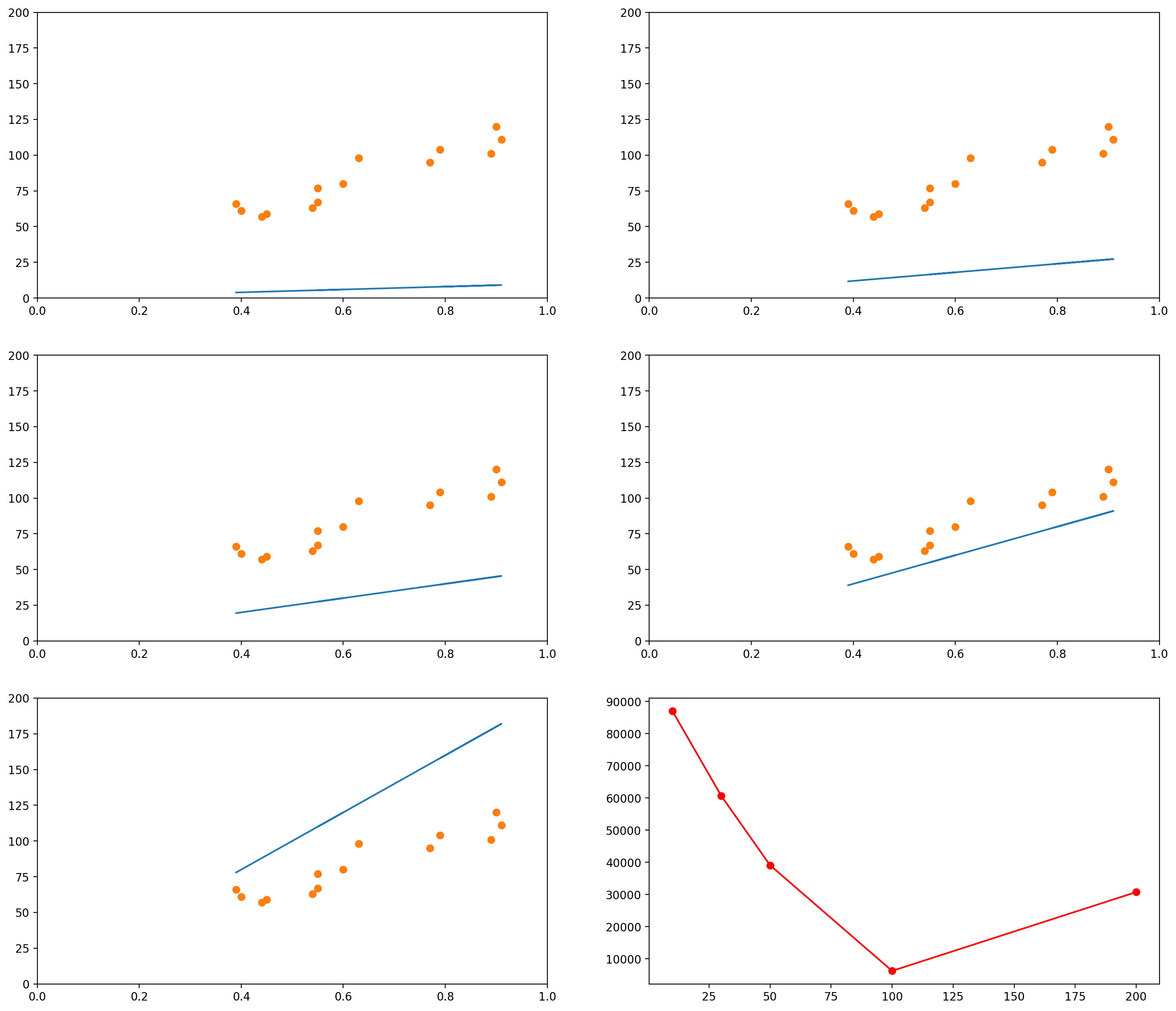
As you can see, when the slope is 10 (the first graph, and the leftmost data point in the last graph), the $L_2$ norm of the error vector is very high. As the slope keeps increasing, the error goes on decreasing, until a certain moment (somewhere between the slopes 100 and 200), when it increases again.
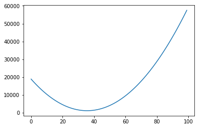
We could plot the Sum of Squared errors of many many of these lines, and we would get a function that looks like the following:
# Initialize an empty list
error_l2_norms = []

for i in range(200):
    # Gets the y values of the line, given the slope i
    plot_y1 = i*plot_x1 + 0
    # Calculates the sum of squared errors for all the data points we have
    sum_squared_errors = sum((plot_y1 - total_reading_time)**2)
    # Inserts the sum in our list
    error_l2_norms.append(sum_squared_errors)

# Now we plot the 200 elements of the list, along with the sum of squared errors
plt.plot(range(200), error_l2_norms)
[<matplotlib.lines.Line2D at 0x7f151446d898>]
Notice that so far we only moved the slope. We could do the same with the intercept. For example, let’s say we fixed our slope in 75. Then we could generate graphs with intercepts, say, 0, 20, 40, 60, 80:
# This is the original data
data_x = mean_pupil_dilation
data_y = total_reading_time
slope = 75

# Let's create some possible lines
plot_x1 = mean_pupil_dilation
plot_y1 = slope*plot_x1 + 0

plot_x2 = mean_pupil_dilation
plot_y2 = slope*plot_x2 + 20

plot_x3 = mean_pupil_dilation
plot_y3 = slope*plot_x3 + 40

plot_x4 = mean_pupil_dilation
plot_y4 = slope*plot_x4 + 60

plot_x5 = mean_pupil_dilation
plot_y5 = slope*plot_x5 + 80

plt.figure(figsize=(18, 16), dpi= 200)

plt.subplot(3,2,1)
plot_line_and_dots([plot_x1, plot_y1], [data_x, data_y], [[0,1],[0, 200]])

plt.subplot(3,2,2)
plot_line_and_dots([plot_x2, plot_y2], [data_x, data_y], [[0,1],[0, 200]])

plt.subplot(3,2,3)
plot_line_and_dots([plot_x3, plot_y3], [data_x, data_y], [[0,1],[0, 200]])

plt.subplot(3,2,4)
plot_line_and_dots([plot_x4, plot_y4], [data_x, data_y], [[0,1],[0, 200]])

plt.subplot(3,2,5)
plot_line_and_dots([plot_x5, plot_y5], [data_x, data_y], [[0,1],[0, 200]])

# Finally, in the last plot, let's look at the error between the

squared_errors1 = (plot_y1 - total_reading_time)**2
squared_errors2 = (plot_y2 - total_reading_time)**2
squared_errors3 = (plot_y3 - total_reading_time)**2
squared_errors4 = (plot_y4 - total_reading_time)**2
squared_errors5 = (plot_y5 - total_reading_time)**2

plt.subplot(3,2,6)
plt.plot([0, 20, 40, 60, 80],
         [sum(squared_errors1),
          sum(squared_errors2),
          sum(squared_errors3),
          sum(squared_errors4),
          sum(squared_errors5)], '-ro')
[<matplotlib.lines.Line2D at 0x7f151437a4e0>]
Of course, again, we could plot the errors of curves for many other values of intercept:
# Initialize an empty list
error_l2_norms = []
slope = 75

for i in range(100):
    # Gets the y values of the line, given the slope i
    plot_y1 = slope*plot_x1 + i
    # Calculates the sum of squared errors for all the data points we have
    sum_squared_errors = sum((plot_y1 - total_reading_time)**2)
    # Inserts the sum in our list
    error_l2_norms.append(sum_squared_errors)

plt.plot(range(100), error_l2_norms)
[<matplotlib.lines.Line2D at 0x7f1514243198>]
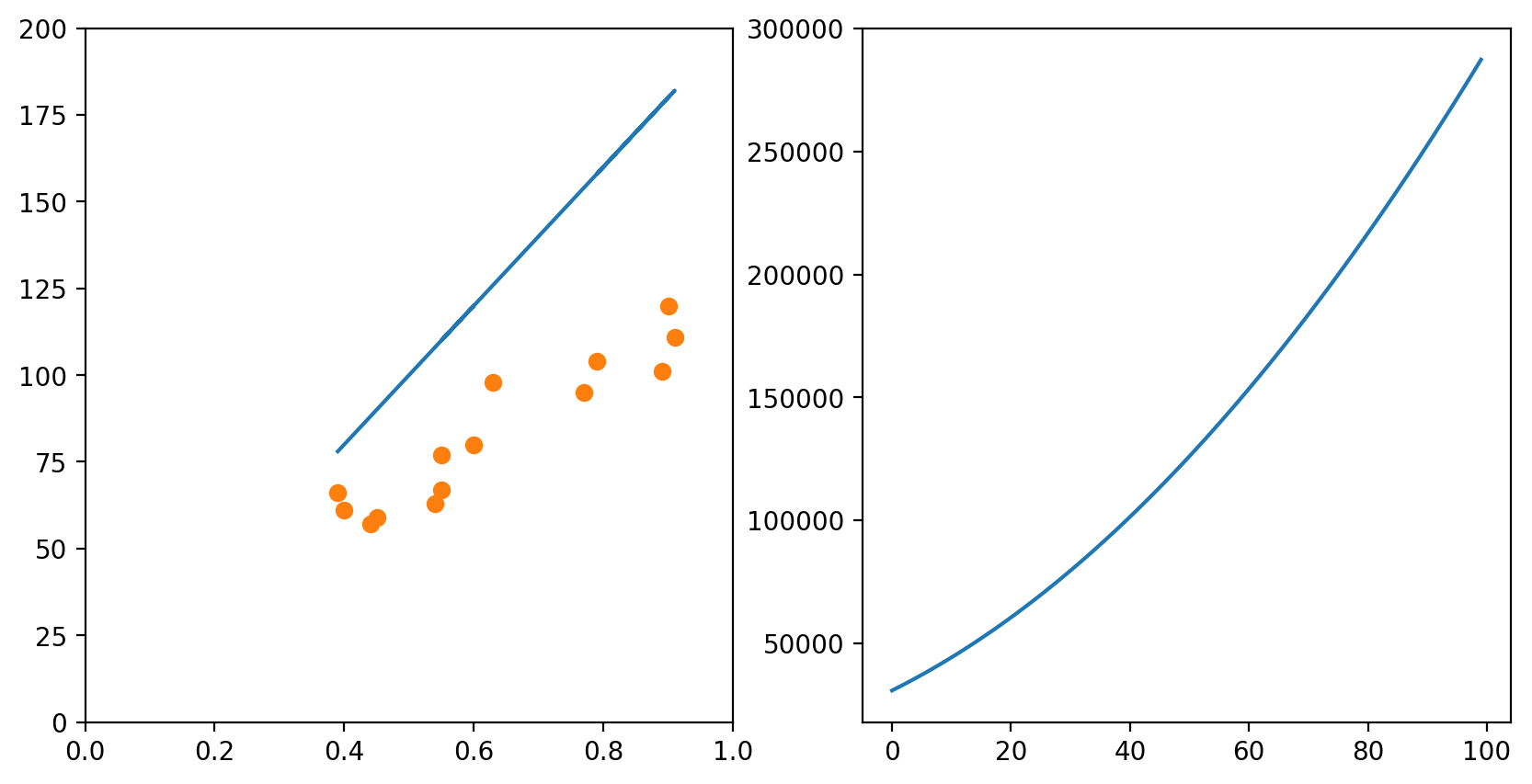
In each of the graphs above, we fixed a value for one of the variables (either the intercept or the slope) and iterated through many possible values of the other variable. It is important to notice that, as one of the variables change, the curve for the other variable also changes. In the example above, we had chosen a slope of 75. The example below shows what happens when we use a slope of 200. The graph to the left has an intercept of 0; the graph to the right shows how the error change as the intercept increases from 0 to 100.
slope = 200

# Change the default size of the plotting
plt.figure(figsize=(10, 5), dpi= 200)

plot_x = mean_pupil_dilation
plot_y = slope*plot_x5 + 0
plt.subplot(1,2,1)
plot_line_and_dots([plot_x, plot_y], [data_x, data_y], [[0,1],[0, 200]])

# Initialize an empty list
error_l2_norms = []

for i in range(100):
    # Gets the y values of the line, given the slope i
    plot_y1 = slope*plot_x1 + i
    # Calculates the sum of squared errors for all the data points we have
    sum_squared_errors = sum((plot_y1 - total_reading_time)**2)
    # Inserts the sum in our list
    error_l2_norms.append(sum_squared_errors)

# Now we plot the 100 elements of the list, along with the sum of squared errors
plt.subplot(1,2,2)
plt.plot(range(100), error_l2_norms)
[<matplotlib.lines.Line2D at 0x7f1515de7c18>]
Of course, if one had time, one could try all possible combinations of slope and intercept and choose the best one. This would generate a surface in the 3D space:
# Initialize an empty list
error_l2_norms = np.zeros([100, 100])

for i in range(100):
    for slope in range(100):
        # Gets the y values of the line, given the slope i
        plot_y1 = slope*plot_x1 + i
        # Calculates the sum of squared errors for all the data points we have
        sum_squared_errors = sum((plot_y1 - total_reading_time)**2)
        # Inserts the sum in our list
        error_l2_norms[i, slope] = sum_squared_errors

X = np.arange(0, 100, 1)
Y = np.arange(0, 100, 1)
X, Y = np.meshgrid(X, Y)
Z = error_l2_norms

fig = plt.figure()
ax = fig.gca(projection='3d')
ax.set_xlabel('Intercept')
ax.set_ylabel('Slope')
ax.set_zlabel('Sum of Squared Errors')
surf = ax.plot_surface(X, Y, Z, cmap=cm.coolwarm, rstride=10, cstride=10)
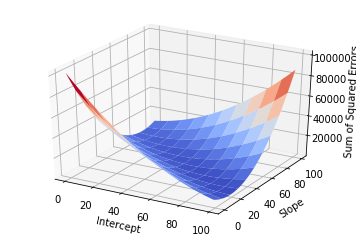
But this approach would be too computationally intensive, and if you had more variables it would probably take too long.
Enter Gradient Descent
To solve this problem in an easy way, we use Gradient Descent. We will first understand the intuition of Gradient Descent, and then I will show the maths.
Using our example above, let’s focus on what Gradient Descent would do if we had the two variables Intercept and Slope and wanted to find the best configuration of Intercept and Slope (i.e., the configuration for which the error is minimum). Gradient Descent would start with any random configuration. Then, given this configuration, it would ask:
- In which direction (and how ‘strongly’) do I need to change my Intercept so that my error would increase?”
In more fancy mathy terms, it would calculate the derivative2 of the error function (the surface plotted above) with respect to the variable Intercept. It would then keep this “direction” in a variable.
At the same time, it would also ask:
- In which direction (and how ‘strongly’) do I need to change my Slope so that my error would increase?”
Again, this is the same as calculating the derivative of the error function with respect to the Slope. It would then also store this “direction” in a variable.
Finally, it would take the current Intercept and Slope and update them using the values it just calculated. But there is a catch: since it calculated the direction in which the error would increase, it updates the two variables in the opposite direction.
More formally
Now we are ready to understand the formal notation for the algorithm. Remember that our error function is the Sum of Squared Errors, also referred to as the $L_2$-norm of the error vector $\boldsymbol{\epsilon}$, and that this $L_2$-norm is normally written as $| \cdot |_2$3. That is, the $L_2$-norm of $\boldsymbol{\epsilon}$ is normally written $| \boldsymbol{\epsilon} |_2$.
Proceeding, we want to represent the derivative of the error function with respect to the variables Intercept (which we were referring to as $A$) and Slope (which we were referring to as $b$). These derivatives are normally written as
\[\frac{\partial \|\boldsymbol{\epsilon}\|_2}{\partial A} \text{ and } \frac{\partial \|\boldsymbol{\epsilon}\|_2}{\partial b}\]Notice that the error function $| \boldsymbol{\epsilon} |_2$ depends exclusively on these two variables. This leads us to the concept of “Gradient”. The Gradient of the error function is a vector containing the derivative of each of the variables on which it depends. Since $|\boldsymbol{\epsilon}|_2$ depends only on $A$ and $b$, the Gradient of $|\boldsymbol{\epsilon}|_2$ (we represent it by $\nabla |\boldsymbol{\epsilon}|_2$) is the following vector:
\[\nabla \|\boldsymbol{\epsilon}\|_2 = \Big(\frac{\partial \|\boldsymbol{\epsilon}\|_2}{\partial A} , \frac{\partial \|\boldsymbol{\epsilon}\|_2}{\partial b}\Big)\]After calculating the value of the Gradient, we can just update the value of $A$ and $b$ accordingly:
\[A \leftarrow A - \lambda \cdot \frac{\partial \|\boldsymbol{\epsilon}\|_2}{\partial A} \\ b \leftarrow b - \lambda \cdot \frac{\partial \|\boldsymbol{\epsilon}\|_2}{\partial b}\]The $\lambda$ there is the “learning rate”. It is just a number multiplying each of the elements of the Gradient. The idea is that it might make sense to make smaller or bigger jumps if you know you are too close or too far away from a good configuration of parameters.
Problems with Gradient Descent
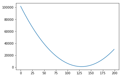
The Gradient Descent procedure will normally help us find a so-called “local minimum”: a solution that is better than all solutions nearby. Consider, however, the graph below:
# Defines (x,y) coordinates for many points for the curve
x = np.linspace(-30, 10, 200)
y = np.sin(0.5*x) + .3*x + .01*x**2

# Plots the (x,y) coordinates defined above
plt.plot(x, y)

# Plots a red dot at the point x=3
plt.plot([3], [np.sin(0.5*3) + .3*3 + .01*3**2], 'ro')
[<matplotlib.lines.Line2D at 0x7f15141414e0>]
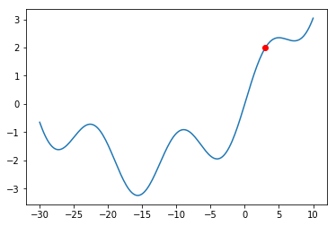
What would happen if we were at the red dot and used Gradient Descent to find a solution? The algorithm might get stuck in the local minimum immediately to its right (near $x = -5$), and never manage to find the global minimum (around $x = 15$). You should always keep this in mind when using Gradient Descent.
Even though there might be shortcomings to Gradient Descent, this is the method used in a lot of Machine Learning problems, and this is why I am introducing it here. The problem of Linear Regression is very often a “convex optimization problem”, which means it doesn’t have those local minima above.
Going beyond 1-dimensional inputs
Of course, the same concepts can be applied when you have more than one variables and you would like to predict the value of another variable. For example, let’s say we now had both the mean_pupil_dilation and the number of fixations (num_fixations below) and we wanted to predict the total_reading_time. In the code below, we will put these values in convenient data structures:
# This was how we had taken the variables separately
mean_pupil_dilation = np.array(data)[:, 1].astype(float)
total_reading_time  = np.array(data)[:, 2].astype(float)
num_fixations = np.array(data)[:, 3].astype(float)

# We can use the `zip()` function to put them all together again
# `zip()` returns a generator... so we use `list()` to transform it into a list
dilation_fixations = list(zip(mean_pupil_dilation, num_fixations))
print("mean_pupil_dilation", mean_pupil_dilation)
print("--")
print("num_fixations", num_fixations)
print("--")
print("dilation_fixations", dilation_fixations)
mean_pupil_dilation [0.9  0.89 0.79 0.91 0.77 0.63 0.55 0.6  0.55 0.54 0.45 0.44 0.4  0.39]
--
num_fixations [20. 18. 24. 19. 20. 22. 30. 23. 56. 64. 42. 43. 51. 40.]
--
dilation_fixations [(0.9, 20.0), (0.89, 18.0), (0.79, 24.0), (0.91, 19.0), (0.77, 20.0), (0.63, 22.0), (0.55, 30.0), (0.6, 23.0), (0.55, 56.0), (0.54, 64.0), (0.45, 42.0), (0.44, 43.0), (0.4, 51.0), (0.39, 40.0)]
Let’s also plot the data in 3D, to get a notion of how it looks like (it is the same data… even though it might not seem the same at a first glance).
fig = plt.figure()
ax = fig.add_subplot(111, projection='3d')

ax.scatter(total_reading_time, mean_pupil_dilation, num_fixations)
ax.set_xlabel('Total Reading Time')
ax.set_ylabel('Mean Pupil Dilation')
ax.set_zlabel('Number of Fixations')
Text(0.5,0,'Number of Fixations')
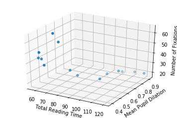
So now, with two input dimensions and one output dimension, we don’t only have a line, characterized by a single slope and a single intercept, but a plane, characterized by 3 variables: one intercept and two coefficients.
In the sections above, our line equation looked like this:
\[\mathbf{y} = A\mathbf{x} + b + \boldsymbol{\epsilon} \\\]Where $A$ was a scalar (a number) and $\mathbf{x}$ was a column vector. That is, the equation looked like this:
\[\begin{bmatrix} y_1 \\ y_2 \\ \vdots \\ y_n \end{bmatrix} = A \begin{bmatrix} x_1 \\ x_2 \\ \vdots \\ x_n \end{bmatrix} + b + \begin{bmatrix} \epsilon_1 \\ \epsilon_2 \\ \vdots \\ \epsilon_n \end{bmatrix}\]Now, instead of having only one $A$, we have two values: $A_1$ and $A_2$. The first value, $A_1$, should be multiplied by the pupil dilation; and the second value, $A_2$, should be multiplied by the number of fixations.
To make this equation function exactly in the same way as before, we can write it like this:
\[\begin{bmatrix} y_1 \\ y_2 \\ \vdots \\ y_n \end{bmatrix} = \begin{bmatrix}A_1 & A_2 \end{bmatrix} \begin{bmatrix} x_{11} & x_{12} \\ x_{21} & x_{22} \\ \vdots & \vdots \\ x_{n1} & x_{n2} \end{bmatrix}^{\top} + b + \begin{bmatrix} \epsilon_1 \\ \epsilon_2 \\ \vdots \\ \epsilon_n \end{bmatrix}\]Of course, if you had more variables, you could just add more columns to the $A$ matrix and to the $\mathbf{x}$ matrix. For example, if you had $m$ variables, you would have:
\[\begin{bmatrix} y_1 \\ y_2 \\ \vdots \\ y_n \end{bmatrix} = \begin{bmatrix}A_1 & A_2 & \cdots & A_m \end{bmatrix} \begin{bmatrix} x_{11} & x_{12} & \cdots & x_{1m} \\ x_{21} & x_{22} & \cdots & x_{2m} \\ \vdots & \vdots & \ddots & \vdots \\ x_{n1} & x_{n2} & \cdots & x_{nm} \end{bmatrix}^{\top} + b + \begin{bmatrix} \epsilon_1 \\ \epsilon_2 \\ \vdots \\ \epsilon_n \end{bmatrix}\]So, putting the numbers in place, remember that we had the following two vectors:
- Pupil dilations: $\begin{bmatrix}0.9 & 0.89 & 0.79 & 0.91 & 0.77 & 0.63 & 0.55 & 0.6 & 0.55 & 0.54 & 0.45 & 0.44 & 0.4 & 0.39\end{bmatrix}$
- Number of fixations: $\begin{bmatrix}20 & 18 & 24 & 19 & 20 & 22 & 30 & 23 & 56 & 64 & 42 & 43 & 51 & 40 \end{bmatrix}$
Then our equation would become:
\[\begin{bmatrix} 66 \\ 61 \\ 57 \\ 59 \\ 63 \\ 67 \\ 80 \\ 77 \\ 98 \\ 95 \\ 111 \\ 104 \\ 101 \\ 120 \end{bmatrix} = \begin{bmatrix} A_1 & A_2 \end{bmatrix} \begin{bmatrix} 0.9 & 20 \\ 0.89 & 18 \\ 0.79 & 24 \\ 0.91 & 19 \\ 0.77 & 20 \\ 0.63 & 22 \\ 0.55 & 30 \\ 0.6 & 23 \\ 0.55 & 56 \\ 0.54 & 64 \\ 0.45 & 42 \\ 0.44 & 43 \\ 0.4 & 51 \\ 0.39 & 40 \\ \end{bmatrix}^{\top} + b + \boldsymbol{\epsilon}\]Just to make it clear, that “$\top$” over the matrix containing our numbers indicates that the matrix was transposed. You could rewrite the equation as:
\[\begin{bmatrix} 66 \\ 61 \\ 57 \\ 59 \\ 63 \\ 67 \\ 80 \\ 77 \\ 98 \\ 95 \\ 111 \\ 104 \\ 101 \\ 120 \end{bmatrix} = \\ \begin{bmatrix} A_1 & A_2 \end{bmatrix} \begin{bmatrix} 0.9 & 0.89 & 0.79 & 0.91 & 0.77 & 0.63 & 0.55 & 0.6 & 0.55 & 0.54 & 0.45 & 0.44 & 0.4 & 0.39 \\ 20 & 18 & 24 & 19 & 20 & 22 & 30 & 23 & 56 & 64 & 42 & 43 & 51 & 40 \end{bmatrix} + b + \boldsymbol{\epsilon}\]Then our gradient descent does exactly the same. We first calculate the gradient of the error function, which now is composed by three elements:
\[\nabla \|\boldsymbol{\epsilon}\|_2 = \Big(\frac{\partial \|\boldsymbol{\epsilon}\|_2}{\partial A_1} , \frac{\partial \|\boldsymbol{\epsilon}\|_2}{\partial A_2} , \frac{\partial \|\boldsymbol{\epsilon}\|_2}{\partial b}\Big)\]And update our variables in the opposite direction:
\[A_1 \leftarrow A_1 - \lambda \cdot \frac{\partial \|\boldsymbol{\epsilon}\|_2}{\partial A_1} \\ A_2 \leftarrow A_2 - \lambda \cdot \frac{\partial \|\boldsymbol{\epsilon}\|_2}{\partial A_2} \\ b \leftarrow b - \lambda \cdot \frac{\partial \|\boldsymbol{\epsilon}\|_2}{\partial b}\]Or, more generally, if we had $m$ variables,
\[\nabla \|\boldsymbol{\epsilon}\|_2 = \Big(\frac{\partial \|\boldsymbol{\epsilon}\|_2}{\partial A_1} , \frac{\partial \|\boldsymbol{\epsilon}\|_2}{\partial A_2} , \dots , \frac{\partial \|\boldsymbol{\epsilon}\|_2}{\partial A_m} , \frac{\partial \|\boldsymbol{\epsilon}\|_2}{\partial b}\Big)\]and updates:
\[A_1 \leftarrow A_1 - \lambda \cdot \frac{\partial \|\boldsymbol{\epsilon}\|_2}{\partial A_1} \\ A_2 \leftarrow A_2 - \lambda \cdot \frac{\partial \|\boldsymbol{\epsilon}\|_2}{\partial A_2} \\ \dots \\ A_m \leftarrow A_m - \lambda \cdot \frac{\partial \|\boldsymbol{\epsilon}\|_2}{\partial A_m} \\ b \leftarrow b - \lambda \cdot \frac{\partial \|\boldsymbol{\epsilon}\|_2}{\partial b}\]Ok… but how do I do Regression in Python? (using sklearn)
We will use the sklearn library in Python to calculate the Linear Regression for us. It receives the input data (the mean_pupil_dilation vector) and the expected output data (the total_reading_time vector). Then it updates its coef_ and intercept_ variables with the slope and intercept, respectively.
(Importantly, because the problem of Linear Regression is quite simple, it is likely not using Gradient Descent in sklearn)
# Adapted from http://scikit-learn.org/stable/modules/linear_model.html

# from sklearn import linear_model

# LinearRegression() returns an object that we will use to do regression
reg = linear_model.LinearRegression()

# Prepare our data
X = np.expand_dims(mean_pupil_dilation, axis=1)
Y = total_reading_time

# And print it to the screen
print("X: ", X)
print("Y: ", Y)

# Now we use the `reg` object to learn the best line
reg.fit(X, Y)

# And show, as output, the slope and intercept of the learnt line
reg.coef_, reg.intercept_
X:  [[0.9 ]
 [0.89]
 [0.79]
 [0.91]
 [0.77]
 [0.63]
 [0.55]
 [0.6 ]
 [0.55]
 [0.54]
 [0.45]
 [0.44]
 [0.4 ]
 [0.39]]
Y:  [120. 101. 104. 111.  95.  98.  77.  80.  67.  63.  59.  57.  61.  66.]


(array([106.68664055]), 15.649335484366574)
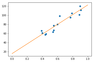
Now we can just plot the line we found using the intercept and slope we found:
# Now we will plot the data
# Define a line using the slope and intercept that we got from the previous snippet
x = np.linspace(0, 1, 100)
y = reg.coef_ * x + reg.intercept_

# Creates the canvas
fig, axes = plt.subplots()

# Plots the dots
axes.plot(mean_pupil_dilation, total_reading_time, 'o')

# Plots the line
axes.plot(x, y)
[<matplotlib.lines.Line2D at 0x7f1513efb898>]
Wrapping Up
Recapitulating, we defined the problem of Regression, defined a (fictitious) dataset on which to base our examples, formulated the problem for one dimension, learned how to evaluate a “solution”, and how this evaluation is used to iteratively find better and better lines (using the Gradient Descent algorithm). Then we expanded the idea for more than one dimension, and finally saw how to do this in Python (actually, we just used a function – which actually probably doesn’t use this method, but, oh, well, the result is what we were looking for).
There is A LOT more to talk about this, but hopefully this was a gentle enough introduction to the topic. In a next post, I intend to cover Logistic Regression. Hopefully, in a third post, I will be able to show how Logistic Regression relates to the artificial neuron.
Very importantly, I think I should mention that this blog post wouldn’t have come into existence if it were not for Kristina Kolesova and Philipp Blandfort, who organized the course of Computational Linguistics in the University along with me, and Shanley Allen, my PhD advisor, who caused us to bring the course into existence. 4
Footnotes
-
I don’t know exactly how the year is divided in the rest of Germany, but here the semesters start in April and October, and are named Summer and Winter semesters, respectively. ↩
-
This is where we need the derivative, that I spoke about when discussing the possible error functions. ↩
-
I noticed that for some reason the blog is showing only one “|” instead of two. I couldn’t find a way to fix this, so I would like ask you to just consider the “|” and the “||” as the same thing. ↩
-
I didn’t ask them for permission to have them mentioned here (I hope this is not a problem). ↩