Arrays and Their Multiple Facets
31 Jan 2018In my first blog post on Convolutions (no need to go read there: this blog post is supposed to be “self-contained”) I discusssed a little about how it would be a good idea to reinterpret the discretized version of the 1D function $f$ as a vector with an infinite number of dimensions. Basically, the only difference between the two ways of viewing this “list of numbers” was that the vector lacked a “reference point”, i.e., the $t$ we had there. Because $f$ was a very nice type of function that was non-zero only for a certain range of $t$’s, we found a way to get this reference point back by dropping the rest of $f$ where $f$ was always zero.
In this blog post, I want to talk about yet another way in which we can look at a vector (and, consequently, at a function $f$). In the next few sections, I will recapitulate the ideas presented in the blog post on Convolutions, explain the other interpretation of vectors, and show how it may be useful when training a classifier.
Arrays Can Be Reinterpreted As Discrete Functions
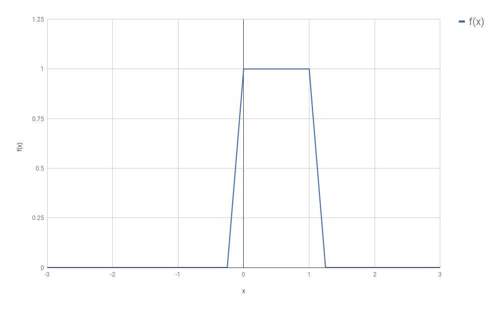
Let’s recapitulate what we learned in the previous blog post. In the example, I had a signal $f$ that looked like the following:
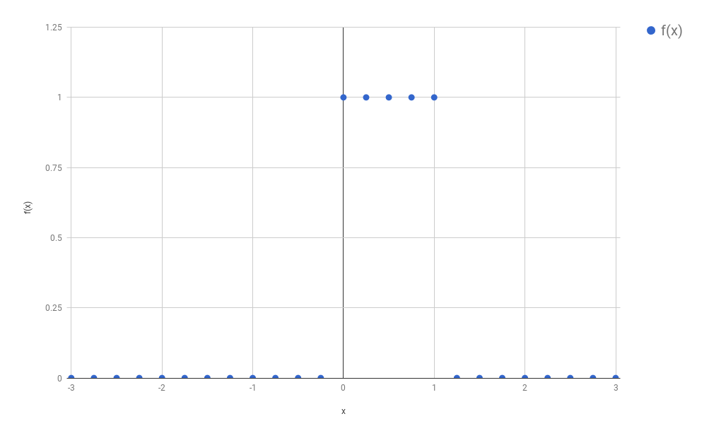
Because we wanted to avoid calculating an integral (the calculation of the convolution, which was the problem we wanted to solve, required the solution of an integral), and because we were not dramatically concerned with numeric precision, we concluded it would be a good approximation to just use a discrete version of this signal. We therefore sampled only certain evenly spaced points from this function, and we called this process “discretization”:
(In our original setting, $f$ was a function that turned out to be composed by non-zero values only in a small part of its domain. The rest was only zeros, extending vastly to the right and to the left of that region. This was convenient for our convolutions, and will be convenient too for our discussion below, although most of the ideas presented below are going to still work if we drop this assumption.)
I would like to introduce some names here, so that I can refer to things in a more unambiguous way. Let $f_{discretized}$ be the newly created function, that came into existence after we sampled several points from $f$, all of which are evenly spaced. Additionally, let us call $s$ the space between each sample. For the purposes of this blog post, we will consider we have any arbitrary $s$. It does not really matter how big or small $s$ is, as long as you (as a human being) feel that the new discrete function you are defining resembles well enough (based on your own notion of “enough”) the original $f$. If you choose an $s$ that is too large, you might end up missing all non-zero points of $f$ (or taking only one non-zero point, depending on where you start). If your $s \to 0$, then you have back the continuous function, and your discretization had basically no effect.
Your new function $f_{discretized}$ now could be seen as a vector composed of mostly zeros, except for a small region:
\[f_{discretized} = [\dots 0, 0, 1, 1, 1, 1, 0, 0, \dots]\]Because this is an infinite array, it is hard to know exactly where it “starts” (or where it “ends”). In the introduction to this post I said this was a “problem”, and we had solved it by dropping the two regions composed exclusively by zeroes:
\[f_{discretized} = [1, 1, 1, 1]\]Of course, we could have retained some of the zeros, if it was for any reason convenient to us. It doesn’t matter much. The main idea here is that we now have a convenient way to represent functions compactly through vectors. This also means that anything that works for vectors (dot products, angles, norms) also should have some interpretation for discrete functions. Think about it!
Disclaiming Interlude
To say the truth, I don’t think that the lack of a “reference point”, as I said before, is a problem at all. From a “maths” perspective, we could solve this by adopting literally any element as our “start”, and from there we can index all other elements. We could even conveniently choose the element that corresponds to our $t = 0$, and it is almost as if we had $f$ back. Mathematicians are quite used to deal with “infinity”, and these seem quite reasonable ideas.
Other human beings, however, would probably not have the same ease, and our machines have unfortunately a limited amount of memory. We would like to keep in our memory only the things we actually care about… and we don’t care a lot about zeros: they kill any number they multiply with, and work as an identity after the sum.
Arrays Can Be Reinterpreted As Distributions
It is very likely that, just by reading the heading of this section, you already got everything you need to know. There is no magic insight in here: I just intend to go through the ideas slowly and make it clear why (and, in some ways, how) the heading is true. If you already got it, I would invite you to skip to the next section, that tries to show examples when the multiple facets of vectors are useful. If you stick to me, however, I hope this section may be beneficial.
What is a Distribution?
When I had a course on Statistics in my Bachelor, it was really bad. At the time of the exam, it seemed I should be much more concerned with how to round the decimal numbers after the comma, than with the actual concepts I was supposed to have learnt. As a consequence, I didn’t understand much of statistics when I started with Machine Learning and it took me a great deal of self-studying to realize some of the things in this blog post.
One of these things was the meaning of the word distribution. This is for me a tricky word, and to be fair I might still miss some of its theoretical details (I just went to Wikipedia, and the article on the topic seems so much more complicated than I’d like it to be). For our purposes here, I will consider a distribution any function that satisfies the following two criteria:
- It is composed exclusively of positive numbers
- The area below the curve sums up to 1
(For the avid reader: I am avoiding the word “integral” because I don’t want to bump into “the integral of a point”, that is tricky and unnecessary here)
There is one more important element to be discussed about distributions: any distribution is a function of one of more random variables. These variables represent the thing we are trying to find the probability of. For example, they might be the height of the people in a population, the time people take to read a sentence, or the age of people when they lose their first tooth.
On Discrete Distributions
(I actually spent a lot of time writing about how continuous distributions could be reinterpreted as vectors, but I have the feeling it was becoming overcomplicated, so I thought I better dedicate one new blog post to my views on continuous distributions)
I believe you should think of Discrete Distributions as the collection of the probabilities that a given random variable assumes any of the values it can assume. For example, let’s say that my random variable $X$ represents the current weather, and that it can be one of the following three possibilities: (1) sunny, (2) cloudy, (3) rainy. Let’s put these three values in a set $\mathcal{X}$, i.e., $\mathcal{X} = \{sunny, cloudy, rainy \}$. Then a probability distribution would tell me all of $P(sunny)$, $P(cloudy)$ and $P(rainy)$. Let’s say that we know the values for these three probabilities:
\[\begin{align*} P(X = sunny) &= 0.7 \\ P(X = cloudy) &= 0.2 \\ P(X = rainy) &= 0.1 \\ \end{align*}\]In that case, it should be easy to conclude that we could represent this probability distribution with the vector $[0.7, 0.2, 0.1]$. Yes! It is this simple! Each one of the outcomes becomes one of the elements of the vector. The ordering is arbitrary. We could have just as well chosen to create a vector $[0.2, 0.7, 0.1]$ from those three values.
But What If My Vector Does Not Sum Up To 1
It may be too easy to transform a distribution into a vector; but what if I have a vector and would like to transform it into a probability distribution? For example, let’s say that I have some computer program that receives all sorts of data (such as the humidity of the air in several sensors, the temperature, the speed of the wind, etc.) and just outputs scores for how sunny, cloudy or rainy it may be. Imagine that one possible vector of scores is $[101, 379, 44]$. Let’s call it $A$. To facilitate the notation, I would like to be able to call the three elements of $A$ by the value of $X$ they represent. So $A_{sunny} = 101$, $A_{cloudy} = 379$, and $A_{rainy} = 44$. If I wanted to transform $A$ into a distribution, then how should I proceed?
There are actually two common ways of doing this. I’ll start by the naïve way, which is not very common, but could be useful if your values are really almost summing up to 1. (Really… they just need some rounding, and you’d like to make this rounding.) In this case, do it the easy way: just divide each number by the sum of all values in $A$:
\[P(X = x) = \frac{A_x}{\sum_{i \in \mathcal{X}}{~A_i}}\]This solution would actually work well for our scores. Let’s see how it works in practice:
\[\begin{align*} P(X = sunny) &= \frac{101}{101 + 379 + 44} = 0.19 \\ \\ P(X = cloudy) &= \frac{379}{101 + 379 + 44} = 0.72 \\ \\ P(X = rainy) &= \frac{44} {101 + 379 + 44} = 0.08 \\ \\ P(X) &= [0.19, 0.72, 0.08] \end{align*}\]While this might seem like an intuitive way of doing things, this is normally not the way people transform vectors into probabilities. Why? Notice that this worked well because all our scores were positive. Take a look at what would have happened if our scores were $B = [10, -9, -1]$:
\[\begin{align*} P(X = sunny) &= \frac{10}{10 - 9 - 1} = \frac{10}{0} \\ \\ P(X = cloudy) &= \frac{-9}{10 - 9 - 1} = \frac{-9}{0} \\ \\ P(X = rainy) &= \frac{-1}{10 - 9 - 1} = \frac{-1}{0} \\ \\ \end{align*}\]
You could argue that I should, then, instead, just take the absolute values of the scores. This would still not work: the probability $P(X=cloudy)$ would be almost the same as $P(X=sunny)$, even though $-9$ seems much “worse” than $10$ (or even worse than $-1$). Take a look:
\[\begin{align*} P(X = sunny) &= \frac{10}{10 + 9 + 1} = \frac{10}{20} \\ \\ P(X = cloudy) &= \frac{ 9}{10 + 9 + 1} = \frac{9}{20} \\ \\ P(X = rainy) &= \frac{ 1}{10 + 9 + 1} = \frac{1}{20} \\ \\ \end{align*}\]So what is the right way? To make things always work, we want to only have positive values in our fractions. What kind of function receives any real number and transforms it into some positive number? You bet well: the exponential! So what we want to do is to pass each element of $B$ (or $A$) through an exponential function. To make things concrete:
\[\begin{align*} P(X = sunny) &= \frac{e^{10}}{e^{10} + e^{-9} + e^{-1}} = \frac{22026.46}{22026.83} = 0.99998 \\ \\ P(X = cloudy) &= \frac{e^{-9}}{e^{10} + e^{-9} + e^{-1}} = \frac{0.0001234}{22026.83} = 0.0000000056 \\ \\ P(X = rainy) &= \frac{e^{-1}}{e^{10} + e^{-9} + e^{-1}} = \frac{0.3679}{22026.83} = 0.0000167 \\ \\ \end{align*}\]The exponential function does amplify a lot the discrepancy between the values (now $sunny$ has probability almost 1), but it is the common way of transforming real numbers into a probability distribution:
\[P(X = x) = \frac{\exp({A_x})}{\sum_{i \in \mathcal{X}}{~\exp({A_i})}}\]This formula goes by the name of softmax and you should totally get super used to it: it appears everywhere in Machine Learning!
Ok… but… so what? How is this even useful?
More or less at the same time I was writing this blog post, I was preparing some class related to Deep Learning that I was supposed to present at the University of Fribourg (in November/2017). I thought it would be a good idea to introduce the exact same discussion above to the people there. When I reached this part of the lecture, it became actually quite hard to find good reasons why knowing all of the above was useful.
One reason, however, came to my mind, that I liked. If you know that the vector you have is a distribution (i.e., if you are able to interpret it this way), then all of the results you know from Information Theory should automatically apply. Most importantly, the discussion above should be able to justify why you would like to use the Cross-Entropy as a loss function to train your neural network. To make things clearer, let’s say that you were given many images of digits written by hand (like those I referred to in my previous blog post):
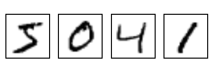
Now let’s say that you wanted to train a neural network that, given any of these
images, would output the “class” that it belongs to. For example, in the image
above, the first image is of the “class” 5, the second image is of the the
class 0, and so on. If you are used to
backpropagation
then you would (probably thoughtlessly) write your code using something like
the categorical_crossentropy of
tflearn (or anything
equivalent). This function receives the output of the network (the values
“predicted” by the network) and the expected output. This expected output is
normally a one-hot encoded vector,
i.e., a vector with zeros in all positions, except for the position
corresponding to the class of the input, where it should have a 1. In our
example, if the first position corresponds to the class 0, then every time we
gave a picture of a 0 to the network we would also use, in the call to our loss
function, a one-hot encoded vector with a 1 in the first position. If the second
position corresponded to the class 1, then every time we gave a picture of a 1
to the network we would also give a one-hot encoded vector with a 1 in the
second position to our loss function.
If you look at these two vectors, you will realize that both of them can be interpreted as probability distributions: the “predicted” vector (the vector output by the network) is the output of a softmax layer; and the “one-hot” encoded vector always sums up to 1 (because it has zeros in all positions except one of them). Since both of them are distributions, then we can calculate the cross-entropy $H(expected, predicted)$ as
\[H(expected, predicted) = - \sum_i{expected_i \log(predicted_i)}\]and this value will be large when the predicted values are very different from the expected ones, which sounds like exactly what we would like to have as a loss function.
Conclusion
Everything discussed in this blog post was extremely basic. I would have been very thankful, however, if anyone had told me these things before. I hope this will be helpful to people who are starting with Machine Learning.