Convolutions and Neural Networks

In my last blog post, I took you by the hand and guided you through the realm of convolutions. I hope to have made it clear why it makes sense to discretize functions and represent them as vector, and how to calculate the convolution of 1D and 2D vectors.

In this post I want to talk a little about how Image Processing was done in the old times, and show the relation between the procedures performed back then and the kinds of parameters learnt by Convolutional Neural Networks (CNN). In fact, do notice that CNNs have been lurking around for years (LeNet had been introduced in 1998!) before they went viral again in 2012 (with the AlexNet), so, in a way, they are concurrent models to the models described below.

It is hard to tell why Convolutional Neural Networks took so long to become popular. One reason might be that Neural Networks had gone somewhat out of fashion for a while until their revival some years ago. (Hugo Larochelle commented in this TEDx video how there were papers that were rejected simply based on the argument that his approach used Neural Networks.)

Another contributing factor might be that, for a long time, it was a common belief for many people that Neural Networks with many layers were not good (despite the work with LSTMs being done in Europe). They were taken as “hard to train” and empirically many experiments ended up producing better performances for models with just a few (or even only one) layer. CNNs, however, did not suffer from these problems (at least not that much), and the LeNet paper from 1998 had already 5 layers.

But my focus here is not on the architecture of CNNs, nor on their gradient flow or their history. My focus here is on how exactly we can say that the shared weights of a CNN results in a mathematical formulation that is identical to that of the Convolutions that we discussed in the previous post.

Image Processing

Before I go into the CNNs I want to show why a Convolutional is something that we might want to do to an image. In my previous post, I tried to be as generic as possible, talking about functions and vectors, speaking from a “signal processing” point of view. It turns out that the Image Processing community has its own perspective. So, from now on, I will take $f$ as a 2D image that I want to somehow process, and to $g$ as a kernel.

When we learn math in school, we learn names of several functions that are known to be useful, and somehow represent well parts of the world we live in. Examples of such functions are $log$, $ln$, $sin$, or $tg$. When we are introduced to statistics, we get acquainted to several other names, such as “correlation”, “standard deviation”, “variance”, “mean” or “mode”. The types of kernels used in Image Processing are not different: researchers in the area have found through the years several kernels that are known to perform well different kinds of tasks, such as blurring, edge detection, sharpening, etc. You can find a list of such kernels in the Wikipedia article.

I want to show how a convolution could be used to find the edges of an image. But this time, I don’t want to show formulas; I think some Python code should make things clearer. Let’s say we want to find the borders of the following image of Lenna:

The first thing to do is to load the image:

from PIL import Image
img = Image.open('lenna.bmp')

Then I want to create a function to convolve the image with the kernel:

# import numpy as np

def convolve(image, kernel):
	# Flips the kernel both left-to-right and up-to-down
	kernel = np.fliplr(np.flipud(kernel))

	# Transforms the image into something that numpy can process
	image_array = np.array(image)

	# Initializes the image I want to return
	new_image_array = np.zeros(image_array.shape)

	# Convolve
	for i in range(image_array.shape[0] - kernel.shape[0]):
		for j in range(image_array.shape[1] - kernel.shape[1]):
			# run_kernel will perform the pointwise multiplication
			# followed by sum
			new_image_array[i][j] = run_kernel(image_array, kernel, i, j)

	# Creates a new Image object
	new_image = Image.fromarray(new_image_array)

	# Returns both the image as an array, and as an Image object
	return new_image_array, new_image

As you can see, I am using numpy to perform the calculations. I expect you not to find it hard to understand the code. It could obviously be written much more efficiently (numpy actually even has a function that performs the convolution anyway), but I wanted to show how the operations we saw in the last blog post can be easily translated into some piece of code.

Now we need to define that run_kernel() function. It calculates the $\odot$ operation between the part of the image that we are interested in and the (already flipped) kernel. This is as simple as:

def run_kernel(image, kernel, pos_x, pos_y):
	ret = 0
	for i in range(kernel.shape[0]):
		for j in range(kernel.shape[1]):
			ret += image[pos_x + i][pos_y + j] * kernel[i][j]

	return ret

Done! It is that simple!

What we are missing is just the right kernel. If you look at the Wikipedia page you’ll see that there are several kernels usable for Edge detection. I’ll use the third one:

In Python:

new_image_array, new_image = convolve(img, np.array([[-1,-1,-1],[-1,8,-1],[-1,-1,-1]]))
new_image.show()

With this, you should see the following image:

Nice, right?

The Border Problem

If you look carefully at this new image, you’ll see that I’m not running run_kernel() in the last pixels (and then you’ll find some columns of zero pixels at the right of the image, as well as some some rows at the bottom). This has to do with what I called the “Border Problem” in my last post.

It is actually very unclear what should be done in the edges of the Image we are trying to process. The way I have been doing so far, if I calculate a convolution between two $3 \times 3$ matrices, it will give me only one number. If you think well about what the size of the final output would be, you will see that it depends on the kernel size. Let’s assume that our final image has $n$ pixels both horizontally and vertically. For a kernel of size $1 \times 1$ (i.e., just a number), the size of the final image would be the same as the size of the original image If the kernel were $2 \times 2$, then the output would have size $n-1 \times n-1$. For a $3 \times 3$ kernel, it would be $n-2 \times n-2$. You can see how this generalizes to $n-(k+1) \times n-(k+1)$, where $k$ is the size of the kernel.

It would be nice if I could find ways to get a result that had the same size of the input image. The most obvious way to do this is to assume that there are zeros beyond the borders of the images. If you think that the images are signals just like the signals from my previous blog post, you should feel that this is a very reasonable assumption to make. Using this assumptions, you will see three types of convolutions:

• Valid: This is the way I have been doing it so far. We don’t assume any information apart from what we have.

• Full: This is the case where we assume there are lots of zeros beyond that the edge of the original image. This way, if we were given the image $f$ below, then it would be “transformed” into the $f_{transformed}$ below before convolving. The number of new rows/columns introduced depends on the size of the kernel. As I said, this should make sense from the perspective of signal processing I described in my previous post. (if this is not clear enough, you are welcome to take a look at this amazing explanation I found in Stack Overflow)

• Same: This is a little trickier. It also assume zeros around the image, but only as much as needed to return an output that has the exact same size as the input image. I tend to find it hard to visualize, but I found that this image helped a lot.

Relation to Convolutional Neural Networks

Ok… so I think we covered everything there was to cover about Convolutions. Now I just need to answer: how do they relate to CNNs?

Remember how the convolutions are being calculated: for a given point in “time”, we multiply the values of both matrices pointwise and then sum them all. Now… remember how the connections of the Convolutional Layer are organized:

Let’s look at one neuron individually. I’d like to call it $a$. It has access to a certain rectangular part of the image. Let’s represent the values of this rectangular part by $A$. So, for example, $A_{0,0}$ represents the element in the leftmost and topmost corner of that rectangular part of the image that our neuron $a$ has access to.

Now, let’s say that $W$ is a matrix with the weights corresponding to the connections between $a$ and the values in $A$. Then the input to $a$ is calculated as

Doesn’t this look a lot like the $\odot$ operation from our kernels? It looks a lot like I am running run_kernel() giving as input the subimage $A$ and the kernel $W$.

Now, let’s focus on another neuron, $b$, and again use a new matrix $B$ to represent the rectangular part of the image that our second neuron has access to. (I hope you see where this is going.) Again, let $V$ denote a matrix composed of the weights of the connections between $b$ and $B$. Then, again, the input to $b$ is calculated as

Again, it looks a lot like I just calculated $B \odot V$, doesn’t it?

If this is hard to see with the formulas, the following image should help a little. It shows the subimages $A$ and $B$, and the connections $W$ and $V$, and how the values are summed when given as input to our neurons $a$ and $b$:

Ok, so now you know that the Convolutional layer is running our $\odot$ operation on small subparts of the image. There is just one last point to be made: Convolutional Neural Networks use shared weights. This means the $W = V$! And this also means that the kernel $W$ (or $V$) is always the same for whichever neuron you choose. This means that if I chose at random any new neuron $c$ to inspect (and defined $C$ as the matrix corresponding to the rectangular part of the input image that $c$ has access to), then the calculation that I would perform would still be

(because, as I said $W = V$!)

In summary, this means that the operation these layers are performing is identical to a Convolution!

Why do we want CNNs?

Now you could ask me: ok, the Image Processing community knows all of these kernels that do magic with my images. Why would I care to have a complex architecture that ends up doing exactly the same kind of thing?

The answer I am going to give is simple, but has huge implications. So far, the Image Processing community had to use their knowledge about how real images generally look like and burn a lot of their own neurons (I mean, figuratively) to generate kernels that somehow fit the problems they were trying to solve. So, if they wanted to find characteristics in the images that would help them to solve the problem they were trying to solve, they had to manually invent kernels that they deemed useful for their task. Many of these kernels followed some patterns/constraints of, e.g., summing up to 1, so that the values of the output image wouldn’t saturate. These patterns somehow limited the types kernels that one could invent, and it was very unintuitive to create anything following different patterns.

But what if, instead of creating kernels by hand (and being bound by constraints, and by our intuition) we could just give a lot of data to a statistical model and just hope that it learns something useful in the end? This is exactly what Convolutional Neural Networks are for. The kernels that are learnt by the CNN are generally not very intuitive, and probably no human would have easily guessed that they are useful for the tasks that these networks are trying to solve (be it classification, of segmentation, or whatever). Still, they have shown great results, and (I would go so far as to say that) the times of “handcrafted feature engineering” are probably over.

Bonus: Shifting a Signal

Before concluding this blog post, I want to show how convolutions can be unexpectedly useful to perform some seemingly unrelated task: the shifting of a signal. I learnt this in the Neural Turing Machines paper and found it a very elegant way of solving the problem. In this section, I’ll go back to my old notation and refer to the 1D signal $f$. Let’s say it is a discrete signals represented by the following vector:

Now let’s say I want to shift all elements of $f$ to the right. How would I do? One way to do it could be to make a “same” convolution of $f$ with a function $g = [1,0,0]$. Let’s see how this would work.

(here, I am taking $t=0$ is when the first element of $f$ is aligned with the element in the center of $g$)

And what if I wanted to shift it to the left? Just use a different function $g = [0, 0, 1]$:

This example should also give an intuition of how convolutions are a good way of processing signals. In the case of the Neural Turing Machines, instead of shifting the signals so “binarily” to the right or to the left, they allow continuous values to the positions of $g$. For example, $g$ could be anything like $[0.8, 0.1, 0.1]$. In that case, most of the signal would be shifted, but part of the information would remain “spread” (“blurred”) through other positions of the signal. While this may be unintuitive, we have seen how unintuitive things may actually be useful for solving some tasks.

Conclusion

I hope to have given a good notion of how CNNs relate to the convolutions we saw in the previous post. My hope is that this will provide a good intuition for how convolutions can be used for other Machine Learning architectures, and allow you to think of convolutions as just some other tool that you can use to solve your problems. As you can see, all of this is very simple, but I wish someone had shown me these ideas when I started learning, instead of having to learn them all by myself. I hope this post makes it easy to extend architectures based on convolutions in a way that is sensible taking into account everything discussed here.

What are Convolutions?

For quite some time already I have been wanting to write this blog post. A little more than one year ago I got acquainted to Convolutional Neural Networks, and it didn’t immediately strike me why they are called that way. I eventually read this blog post that helped a lot to clarify things; but I thought I could try to give more details on what exactly is meant when one says “Convolution” here.

This blog post builds upon the description given there, so, if you still didn’t read that, stop reading this and go there take a look at that blog post. I may overlap some of the discussions here with the discussions there.

In the sections that follow, I’ll introduce convolutions (actually, I’ll let Kahn Academy do that for me), then introduce a procedure to calculate it, motivate a discussion about discrete convolutions, show why it makes sense to represent the convolving functions as vectors and extend the definition to the 2D space. The next blog post will explain why these are useful for signal processing and what is their relation with Convolutional Neural Networks.

Convolutions

Convolutions are a very common operation in signal processing. While the colah’s blog post presents it in a more abstract/intuitive statistical way, I find that a more gore calculus-driven introduction from Kahn Academy might help you realize that the concept is just an integral:

In this Kahn Academy video, Sal found a closed formula for the convolution by solving the integral. Given that a convolution is an integral, you might consider that it represents the area below some curve. But what curve exactly? I’ll discuss more about it in the next section. For now, what is worth is to understand that there several ways in which you can think of convolutions, and it might help a lot if you allow yourself to switch views at different points in time.

A concrete example

If you go to the Wikipedia article on convolutions, you may find the following two (awesome) images:

What these images are saying is that you can calculate the value of the convolution $f \ast g$ at the point $t$ by following a very simple procedure. I’ll define two functions $f$ and $g$ to make the steps easier to follow. Let

and

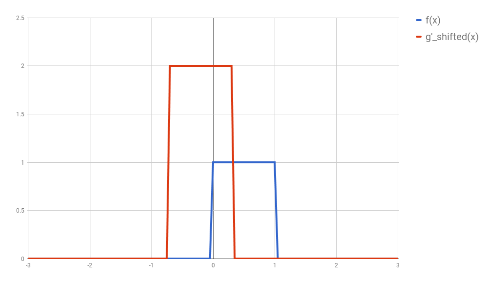
Here we have the two curves:

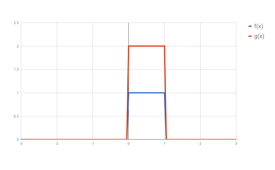
(I used Google Spreadsheets to do this, so you’ll notice the lines are not exact, but you should be able to get the idea)

First: flip $g$ horizontally (i.e., $g(x) <- g(-x)$). Let’s give the flipped $g$ a name, say $g’$. (if you don’t flip $g$, then what you are calculating has actually the name of “cross-correlation”, and is simply another typical operation in signal processing.).

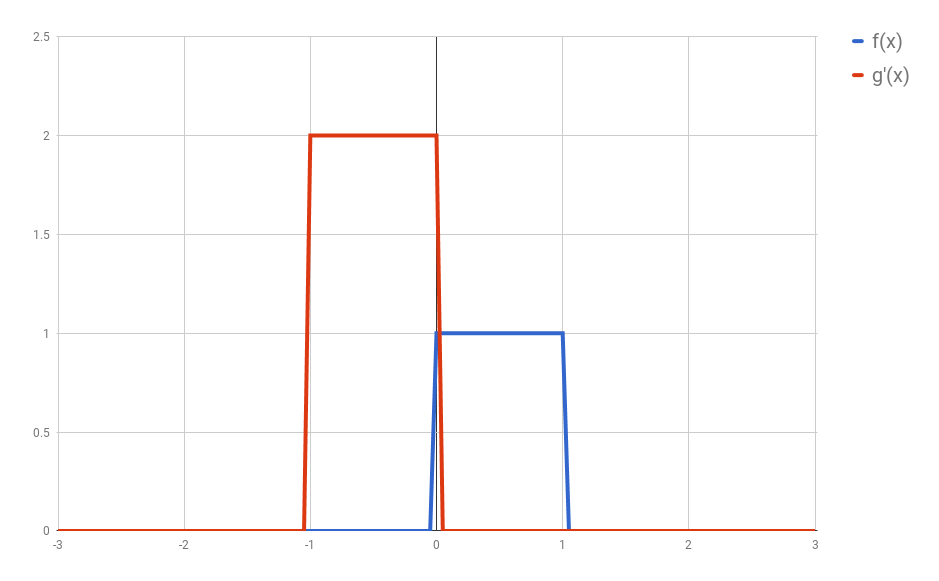
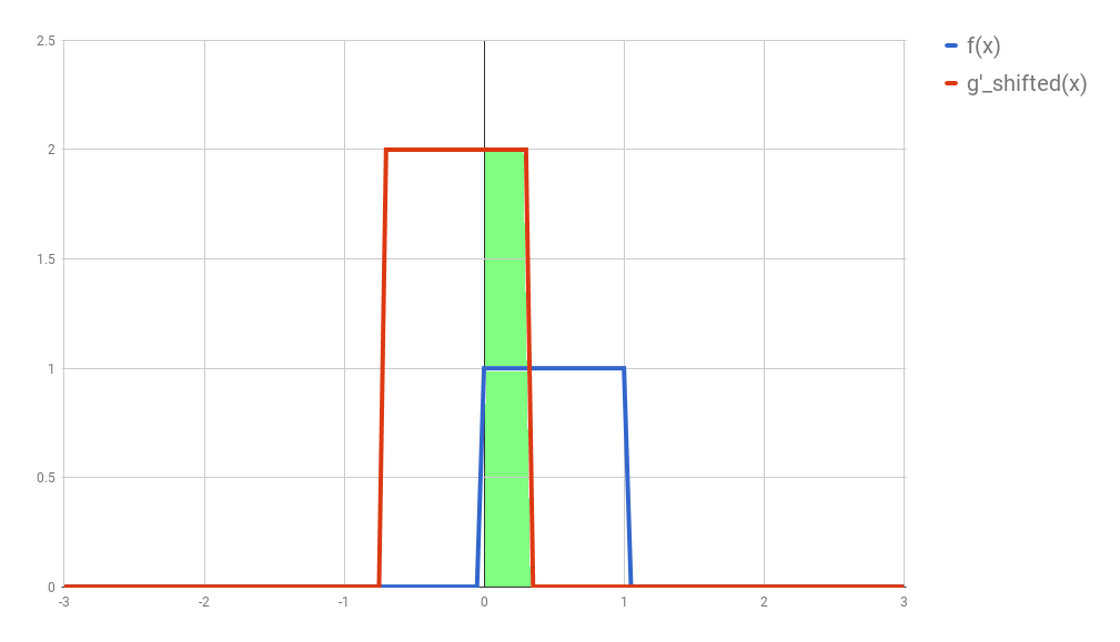
Second: shift $g’$ horizontally by $t$ units. If $t$ is positive, then $g’$ will be shifted to the right; otherwise, it will be shifted to the left. For our example, let’s say that $t=0.3$. I’ll call this function $g_{shifted}’$

Third: this is the step where the problems arise. Now what you want is actually multiply the two curves are each point between $-\infty$ and $+\infty$ and calculate the area below the curve that this multiplication will form. Let’s assume that the functions are zero most of the time (just like in our example), and non-zero only in a small section of their domain. Because we are multiplying the two values, we only care about the values where both functions are not 0. In all other cases, the integral will be 0 anyway. Let’s assume that both functions are non-zero only in an interval $[a, b]$. In this case, our problem reduces to calculating the integral of the multiplication of $f$ and $g_{shifted}’$ inside that interval. Now it could still be a challenge to calculate the integral of the $g_{shifted}’$ and “f” in that interval.

(While searching for a way to understand this procedure, I came across this very nice demo. In it you can define your own functions and play arround to find out how the convolution is going to be.)

The problem with continuous convolutions is that we would have to actually calculate an integral. But what if our function were actually “discrete”? Fortunately for us, most applications on Image Processing require discrete signals, and for our purposes it would be perfectly ok to discretize these continuous signals.

After discretization, All the concepts we have discussed so far would follow the same logic. Now, instead of an integral we now have a sum. So, given the interval $[a, b]$, we could calculate the convolution as

And fortunately this sum is easy to calculate.

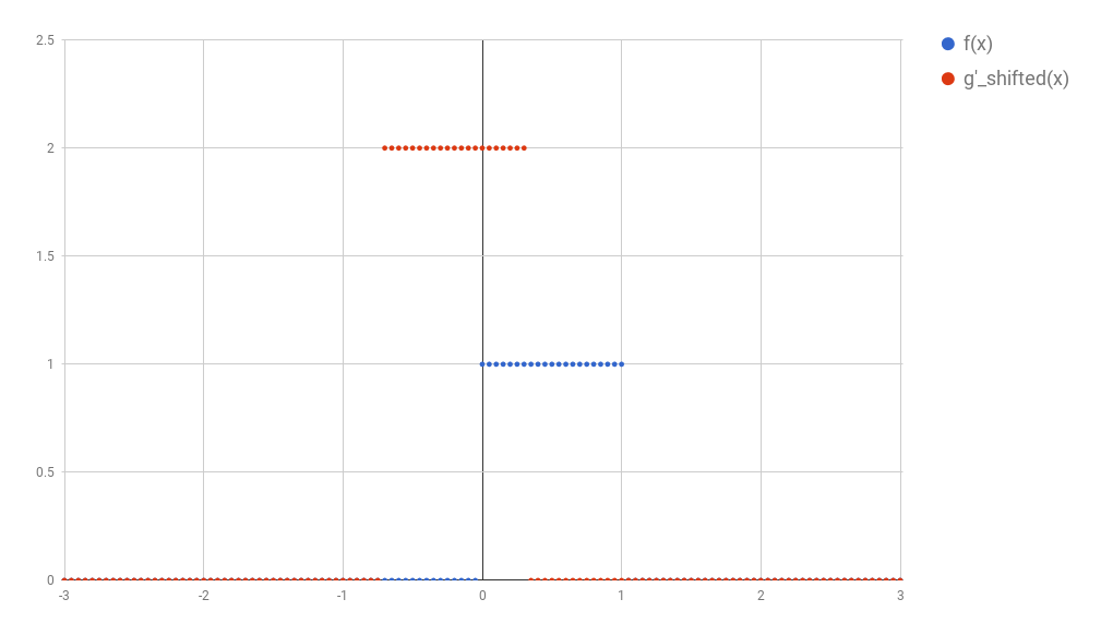
Note: the avid reader may notice that the integral of an interval spanning only a point should have been 0 (and therefore the convolution should always have become 0 after the discretization). The reason why this does not work has to do with the dirac delta function, and I won’t go into many details here. You can just assume that the discretized version of the signal is a sum of dirac delta functions.

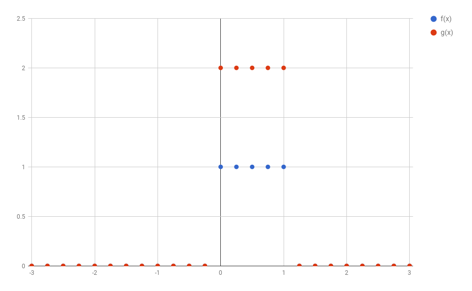
In the example above I discretized the functions using 1 point for each 0.05 step in $x$. This would make the discussion below very hard to understand. So, to make things simpler, in all the text that follows I’ll use steps of 0.25 instead. The image below shows how the original functions $f$ and $g$ would look like discretized this way.

1D discrete convolutions

It turns out that the functions $f$ and $g$ used in convolutions are in reality most of the times composed almost entirely by zeros (as assumed before). This allows for a much more compact representation of the functions as a vector of values. For example, $f$ and $g$ could be represented as:

\(f = [\dots 0, 0, 1, 1, 1, 1, 0, 0, \dots] \\ g = [\dots 0, 0, 2, 2, 2, 2, 0, 0, \dots] \\\) (Of course, the number of 1 and 2 depends on how the discretization was performed)

Now let’s say I’d like to calculate the value of the convolution between $f$ and $g$ at the point $t = $some coordinate. It is hard to point the exact place, so I’ll make the place bold:

\(f = [\dots 0, 0, 1, 1, \textbf{1}, 1, 0, 0, \dots] \\\) (For future reference, I’ll call this position $t=2$)

The way to calculate it is just the same:

• Flip $g$ (but it has no effect here, because $g$ is symmetric anyway);

• Move $g$ horizontally by $t$: this is a little abstract here; but if we align the $f$ and $g$ the way they were initially aligned, then we should get:

• Multiply all elements position by position and sum them all.

You might have noticed how these operations may resemble dot-products. You could have implemented them as:

This way, if you wanted to calculate the convolution for many different values of $t$, you could just keep shifting the vector $g$.

Unfortunately, these are still vectors with an infinite number of dimensions, which are hard to store in our limited storage computers. It is worth noting that very often the functions $f$ and $g$ for which we want to calculate a convolution are 0 most of the time. Since we know that the result of the convolution in these regions will be zero, we can just drop all of the zeros:

\(\begin{align*} f &= [0, 0, 0, 0, 1, 1, 1, 1, 0, 0] \\ g &= [0, 0, 0, 0, 2, 2, 2, 2, 0, 0] \\ (f \ast g) &= [0, 2, 4, 6, 8, 6, 4, 2, 0, 0] \\ \end{align*}\) (As you can see, I kept some of the zeros. I could have removed them. It was my choice)

And congratulations, we just arrived in a very compact representation of our functions.

Note: The entire discussion so far supposed that we would keep $f$ still and always transform $g$ according to our three steps to calculate the convolutions. It turns out that convolutions are commutative, and therefore the entire procedure would have also worked by holding $g$ still and changing $f$ in the same way. (Incidentally, they are also associative)

But what does all of this mean?

When I started talking about convolutions, I said that they are used a lot in the context of signal processing. It might be a good idea to forget that these vectors are functions for a while and consider them signals. (this video might help to convince you that this is a sensible idea.) In that case, what a convolution is doing is taking two signals as input and generating a new one based on those two. How the new signal looks like depends on where both signals are non-zero. In the next blog post you’ll see how this can be used in meaningful ways, like finding borders in an image, blurring an image, or even shifting a signal in a certain direction.

Most importantly, convolutions are a very simple operation (composed of sums and multiplications that can be done parallely), which can be easily implemented in hardware. They are a great tool to have in hand when solving difficult problems.

2D Convolutions

It shouldn’t be a big leap to extend these concepts to the 2D space.

Let us skip all the discussion about continuous functions and vectors with infinitely many elements and consider our current state: functions $f$ and $g$ are represented as small vectors, and we want to calculate the convolution of those two functions (vectors) at any point $t$. If we now define new $f$ and $g$ in a 2D space, then we can represent them as matrices. For example, if we now redefine $f$ as

and rediscretize it in the same way we did before, then we would get a matrix that looks something like:

(Do not forget: I was the one who decided to keep a border with zeros. I could have left many more columns and rows with zeros in the borders. This may seem irrelevant for now, but will be useful when we discuss kernels in the next blog post.)

Let us define a new $g$, that after discretization looks like the following:

How would the convolution then be calculated? Same steps:

• Flip the matrix $g$ (both horizontally and vertically), generating $g’$.

• Shift $g’$ (according to the place where you want to evaluate the convolution). Basically, you want to align $g’$ with some part of $f$.

• Multiply the aligned elements and sum their result.

An example calculated by hand

Before concluding this blog post, I want to calculate an example by hand. If you did not understand everything so far, this should clarify whatever is missing. Let’s define two new functions $f$ and $g$, that, after discretization and “vectorization”, become the following matrices:

If you think of $f$ as an image, you might interpret it as two diagonal lines (the values with 6) surrounded by some “shade” (the values with 3). The function $g$, on the other hand, is hard to interpret. I chose a very asymmetric matrix to show how the flipping (the first step in our calculation) affects the final values in $g$.

Let’s calculate $(f \ast g)(0,0)$. First is to flip $g$ to create $g’$:

Then we align the matrix $g’$ with the part of $f$ that corresponds to position $(0,0)$. This part might cause some confusion. Where exactly is $(0,0)$? There is no actual “right answer” to where this point should be after discretization, and we don’t have the original function formula to help us find out. I’ll call this “the border problem” and refer to it in the next blog post. For now, I’ll just align with the points “we know” and forget about any zeros that might lurk beyond the border of the matrix representing $f$. This will give us a so-called “valid” convolution.

Finally, we need to multiply each element pointwise and sum all of the results. To make things clearer, if $A$ and $B$ denoted the two matrices of same size that we now have, then what we want to do is:

Where I am representing this “pointwise multiplication followed by sum” by the operator $\odot$. In our specific case, we get:

Easy, right?

Now to calculate $(f \ast g)(1,0)$ we just move the matrix $g$ to the right, aligning it with the next submatrix of $f$:

And the other two elements are calculated the same way:

Resulting in the final matrix:

Conclusions

In this blog post I expect to have given you a very intuitive understanding of how convolutions are calculated and a notion of what they are doing. It should help you to make the connection between all those integrals you find in Kahn Academy or Wikipedia and the discrete convolution operation you see in some Neural Networks. If none of this still happened, the examples of the next blog post will definitely help you to realize what is going on.

I had not planned for this blog post to become so long. In the next blog post I’ll show applications of convolutions from the image processing field, and how they connect to Convolutional Neural Networks. As a bonus, I want to show a very elegant application of convolutions from the Neural Turing Machines.

Stay tuned =)

UPDATE: Thanks to Fotini Simistira for pointing some mistakes in my calculations.

What is Machine Learning?

When I started getting in touch with Artificial Intelligence (AI), no one could give me a clear distinction between all those buzzwords such as “Artificial Intelligence”, “Pattern Recognition”, “Data Mining” and “Machine Learning” (ML). It took me a long time to actually be able to dintinguish the meaning of these, and, to say the truth, it is still not very clear to me how exactly the first three relate to each other. The meaning of “Machine Learning”, however, is very simple, and I believe it should have been made clearer from day one. This post has the goal of separating “Machine Learning” from this mess, making it very clear when something is ML and when something is not, and what the relation between ML and AI is.

That said, while I do expect you to have a perfect notion of what is and what is not part of the field after you read this blog post, I don’t intend to give you a better definition of the expression “Machine Learning” than the definitions you may have already found in other places in the web.

Why the confusion?

When I sat down to write this blog post, I thought of taking a look at how others have defined the field before (because, of course, I didn’t expect to come up with any magic new definition). I came across this video (from the amazing course on Machine Learning in Coursera by Andrew Ng):

And this video:

If you watch them, you will see these three field definitions:

Field of study that gives computers the ability to learn without being explicitly programmed.

A computer program is said to learn from experience E with respect to some task T and some performance measure P if its performance on T, as measured by P, improves with experience E.

These first two definitions are good, because they make it clear that the programmer doesn’t tell explicitly what the machine should do: the behavior of the machine is completely dependent on the data it has previously seen (and of course the ways in which the machine learns).

"The extraction of knowledge from data"

A problem with this last definition is that it does not clarify who extracts the knowledge from the data. If the programmer writes rules that conform to the patterns in the data, does this count as Machine Learning? (more on this in the next section)

If you look back at these three definitions, they may cause you to be confused about what exactly the relation between Machine Learning and other fields is. Why is it “Machine Learning” and not, say, “Artificial Intelligence”? (and how is it related to AI, in the first place?) And when am I applying AI that is not ML? And can I apply ML that is not AI?

So… how do I explain this?

A simple story

As I said, I don’t actually intend to give any better definition. Any definition I could present here could be probably invalidated after any amount of some more “socratic” scrutinity. Instead, (and following the field itself,) my explanation is based on examples.

Say you are a photographer who takes two types of pictures: (1) landscapes; and (2) people’s faces (say, for their CV). Let’s assume you have them all stored in a folder in your computer. One fine day you decided to organize your pictures into two folders (landscapes and cv). You started dumping some of your stored photos into the two folders, but after some 50000 images you realized they were too many and thought it would be nice to have some automatic method to do that.

In the lack of a better idea, you decide that an easy way to check if the image is of a human is to count the ammount of pixels that have a color similar to a human skin color. You create a rule that says something like “if the image has more than 500 pixels of those colors, then it is a cv picture”.

You write a program that counts the number of pixels of those colors in your images and moves the files to the respective folder. You run your program and realize that you cv folder now has a lot of images of sandy landscapes. Your program did not do what you hoped it would.

You look better at the images you had already classified, trying to find patterns that could help you to identify the two types of images. You make, say, a histogram of the colors in the two types of images and realize that there is a set of rules that you could apply that would work in most of your cases. You implement those rules, run your program, and feel relatively satisfied: you did as well as you could.

Was this AI? Was this ML? (1)

Now… look back at the story and think about it: did you just make AI? I would say that the answer should probably be yes: if your program had worked, someone who has never seen what your program does would have most probably believed your program was “intelligent”. On the other hand, your rules were engineered by you, and the machine was only supposed to apply them to decide what to do. While you may feel you “taught” the machine what it should do in each case, all the teaching was done through “explicit programming” (see the first definition of Machine Learning in the previous section). In other words: it was not the machine who learnt; it was you.

Revisiting your story

You think you could achieve some better performance, but you are not sure exactly how. Instead of simply counting the colors of your pixels and using this to conclude the type of the image, you think it would be a nice idea to use some fancy image processing techniques. You recall something called the “Discrete Fourier Transformation”, that allows you to get a representation of the images in the “frequency domain”. You apply it to some of your already classified, and realize that, truly, the cv pictures have a very specific pattern of frequencies that you can develop some set of rules for… and anything that does not conform to that pattern seem to be a landscape. You implement your algorithm and feel a little more confident that this time there are fewer errors.

Was this AI? Was this ML? (2)

If you think the first version of your “image classifier” was AI, then you should probably take this second version as AI. (One common complaint among AI practitioners is that people stop taking something as AI as soon as they find out how it works).

On the other hand, could you say you just did ML? My answer is still no: it is not because you applied some fancy “feature extraction” algorithm to understand your data that you are now doing Machine Learning. Again, all the extraction of knowledge is done by you, and you just explicitly instructed the machine to follow what you considered to be the best set of rules you could think of.

So… well… then… actually… when is it ML?

Let’s look one last time to your story. You came a long way until here: used some exploratory statistics to find what the colors in each type of images can tell about them, and also what frequency patterns your images most commonly have. You implemented a rule-based classifier that decided in which folder to put each one of your images.

But you feel all of these rules you developed are not good enough. It would be great if the program could learn by itself what folder to put each image in, based on examples of images of each type. Enter Machine Learning!

When you apply Machine Learning, you don’t want to tell what rules to use: you give data, and you expect the program to figure out by itself what to do. For example, let’s say you still have those 50000 images you had manually classified in the beginning of our story. Let’s say you heard of some popular image classification model called Convolutional Neural Network for which you found some code in the internet and would like to try. In this case, for each one of your 50000 “training” images, you also tell the model what is the answer you expect it to give back (i.e., either cv or landscape). When you start, the model makes a lot of mistakes, outputting many times cv when it was supposed to output landscape, and vice-versa. But every time it makes a mistake, it updates its internal variables in a way that causes it to become more likely to answer right the next time. When the model is done training, you should expect it to answer right most of the times (at least for those 50000 images you were using to train it).

Now that it is done training, you put those 50000 images aside and use the already trained model to put all of your other images in their respective folder. Notice that you didn’t tell the model what to look for in each image. You may have told it how to update its internal variables, but you didn’t explicitly develop any rule. The “rules” were found by the model itself. It learned them!

Some final thoughts

Machine Learning is a huge field, and is going through some nice hype in the last few years. The example I gave in the previous subsections uses something called “Supervised Learning”, which is when you tell the model what is the expected answer for each training instance. There are other models for which you don’t have to explicitly point out the “right answer” every time (and that are useful when you don’t have those 50000 manually labeled examples you trained your Convolutional Neural Network with).

The models may also learn several different types of things. In the case of Convolutional Neural Networks, it is actually not 100% clear what the networks are learning; however, other types of models may learn, say, rules, just like those you were trying to develop manually in the beginning of our story.

Other resources

There are a lot of resources in the internet on both AI and ML. There are some, however, that are my favorites, which I thought of linking here.

On Artificial Intelligence:

• The AI Revolution: The Road to Superintelligence There are two parts. I am linking only the first one because the other part is also easy to find there. This post links to A LOT of other nice stuff that I find extremely interesting, like this 1993 essay on the idea of a singularity in AI.

• Artificial Intelligence & Personhood: A video on what could happen if we reach a point when AI becomes good enough. (I am linking the entire playlist because I do think that a lot of the stuff there is absurdly relevant to the topic)

On Machine Learning

• The amazing course on Machine Learning in Coursera by Andrew Ng, that I had already linked before.

• Some nice tutorial on Machine Learning from Google

First Post

Good morning and welcome to the Black Mesa Transit System. This automated train is provided for the security and convenience of the Black Mesa Research Facility personnel. The time is 8:47 AM. Current topside temperature is 93 degrees with an estimated high of 105. The Black Mesa Compound is maintained at a pleasant 68 degrees at all times.

Well… this is a greetings delivered by the Black Mesa Transit System. In the upcoming weeks I intend to have some serious content in this blog, which will hopefully replace this dummy blog post.

In the meanwhile, maybe you could take a look at the Poems and Songs sections in the sidebar =)